This documentation will cover the basics of how a camera processes light captured through sensors using an image signal processing pipeline (ISP) to procude crips, colorful, and compressed images.

I am also posting YouTube tutorials that go in depth in regards to how each step in the pipeline works, as well as how to implement each step in python code.

• Here is the link to the YouTube playlist.
• Here is the link to the bayer domain image I use in the videos, githubs, and this documentation.
• Note, the YouTube videos cover a basic implementation of the ISP while conceptually explaining the fundamental concepts. I have also built a more advanced, fast ISP that utilizes Numpy Vectorization techniques to increase the speed of the pipeline by over 120 times (from ~25 minutes to ~10 seconds). This documentation will cover the fast ISP. Here is the link to my fast ISP github page.

Link to the CMOS sensor video

The CMOS sensor is built of an array of pixels, each with a micro-lens, color filter, and silicon diode.

Incoming light gets focused onto the color filter, and only light of the correct color can pass through the color filter to strike the silicon diode. The photoelectric effect allows for electrons to build up from the light in an electron well. The electrons then create a voltage signal, which is read by a sensor. Here is a link to a basic article I wrote that covers concepts like the photoelectric effect if you need a refresher.

A black and white, checkerboard image is created based on the voltage signals, and color information is stored in the location of the pixel.

This is how different bayer domain images look. The type of bayer image is defined by the color filter of the top-left 2x2 section. Note, the actual Bayer image is black and white and does not have these colorings. The colors are included in the diagram only for clarity.

This is what the raw bayer domain image looks like before any transformations are applied.

Link to the DPC video

A common aspect ratio of 1920 x 1080 p will require a CMOS sensor of over 2 million pixels. Some of these pixels are bound to be broken or otherwise 'dead'. For example, the voltage sensor on a pixel may have gotten disconnedcted from the potential well, so the pixel at this location is always returning a 'measured' voltage of 0.

We detect dead pixels by comparing their values to their surrounding neighbor pixels. If there is a significant difference, we correct the dead pixel by mathematically approximating its value based on the value of its neighbors.

Note, the neighboring pixels are not literally the pixels touching p0, but rather the 8 surrounding pixels of the same 'color' as p0. In the above image, if p0 is a pixel that had a red filter on it, then p1-p8 also had red filters.

The formula we use to detect dead pixels is the following:

Where p0 is the center pixel and px refers to the neighboring pixels.

1. To ensure corner pixels have a full set of neighbors, we pad the image. Then, to vectorize this operation, we create seperate arrays for p0-p8. To emphasize this important point again, p0-p8 are spread across a 5x5 region to ensure they are all representing the same color pixels.
padded_bayer = np.pad(bayer, (2,2), 'reflect') p1 = padded_bayer[:-4:1, :-4:1] p2 = padded_bayer[:-4:1, 2:-2:1] p3 = padded_bayer[:-4:1, 4::1] p4 = padded_bayer[2:-2:1, :-4:1] p0 = padded_bayer[2:-2:1, 2:-2:1] p5 = padded_bayer[2:-2:1, 4::1] p6 = padded_bayer[4::1, :-4:1] p7 = padded_bayer[4::1, 2:-2:1] p8 = padded_bayer[4::1, 4::1]
2. Then, we can create new arrays with the absolute value of the difference between p0 and p1-p8. Anywhere the difference exceeds a given threshold, there is a dead pixel.
neighbors = np.array([p1, p2, p3, p4, p5, p6, p7, p8]) diff = np.abs(neighbors - p0) condition = diff > thresh sum = np.sum(condition, axis = 0)

We now have the array sum, which is an array of the same size as the original bayer image. If the value of sum at a certain index is 0, then the pixel at this index is reasonably similar to its neighboring pixels, and is declared not dead. If sum is greater than 0, the pixel is declared dead.

To correct the dead pixels, one option is to replace the dead pixels with the average value of p1-p8. We can do so simply with the following command:

Another option is to use a gradient based approach that is more sensitive to edges in the image. There are 4 directions that an edge can take that cross through p0 - vertical, horizontal, diagonal right, and diagonal left.

From here, we can compute the average value of the pixels involved in each gradient. For example,

Of the four directional gradients, the one with the minimum value will have the least change in brightness intensity across the given direction, and will therefore be the least likely direction to pass across an edge. Calculating p0 using an average of only this direction's neighbroing pixels will help to avoid edge blurring.

Regardless of which method you choose though, the effects will likely not be visible to the naked eye yet, since there are millions of pixels, and generally very few are dead. However, with a complete pipeline, the effects of each module can be seen easily by removing the modules one at a time and viewing the final results.

Resulting image after applying Dead Pixel Concealment

Link to the BLC video

We would expect that the pixel value for a section of an image that is supposed to be black would be 0. But there will always be light falling on every pixel when a picture is taken, and unless the pixel in question is dead, the photoelectric effect ensures that the returned voltage signal can not be 0.

To address this issue, Black Level Compensation will subtract an offset from each color channel. This offset is usually very small, roughly around 10-50.

1. To apply Black Level Compensation, we first extract each channel using Numpy slicing.
r = dpc_img[::2, ::2] gr = dpc_img[1::2, ::2] gb = dpc_img[::2, 1::2] b = dpc_img[1::2, 1::2]
2. Then, we apply offsets.
r = r + offsets['bl_r'] gr = gr + offsets['bl_gr'] gb = gb + offsets['bl_gb'] b = b + offsets['bl_b']
3. Finally, we recreate the image, again using Numpy slicing.
blc_img[::2, ::2] = r blc_img[1::2, ::2] = gr blc_img[::2, 1::2] = gb blc_img[1::2, 1::2] = b

The image we are currently using is in the uint16 datatype, with values ranging from 0 to 65535. Just like in DPC, the effects of the transformation will not be visible to the naked eye yet. This time, it is since the offset is less than 0.1% of the total range, and the human eye cannot reliably detect such minor changes in light intensity.

Resulting image after applying Black Level Compensation

Link to the LSC video

When a camera takes an image, a majority of the light taken in is focused by the lenses to the center. This leaves the central area of the image much brighter than the outer areas. This phenomenon is called lens shading.

To address this issue, we run a correction algorithm based on radial distance from the center of the image. The formulas is as follows:

Where r is the radial distance form the center of the image, k is a correction factor (very small, usually about 0.0005-0.005), and the offset is an integer.

1. To apply the transformation in Python, we first use Numpy meshgrids to create an array that stores information about each index's distance from the center.
x, y = np.meshgrid(np.arange(cols), np.arange(rows)) radial_dist = np.sqrt((x - center_x)**2 + (y - center_y)**2)
2. We don't want to overdo the correction, resulting in bright outsides and dimmer insides. To prevent this issue, we cap the radial-distance value.
radial_dist = np.where(radial_dist <= 1300, 1300, radial_dist)
3. Finally, we apply the transformation formula to the previously created blc_img, and then rescale all values to be integers.
lsc_img = (blc_img * (k * radial_dist + 1) - offset).astype(np.uint16)

The more extreme that the k value for is, the more easily it is to visualize the effects of LSC. Regardless, unlike previous modules, you can visually start to see the effects of this module even with an average, useful k value.

Resulting image after applying Lens Shading Correction with k = 0.0015

Link to the AAF video

Filters are mathematical or algorithimic expressions applied to images generally on a pixel-by-pixel basis, and they are used for various purposes such as enhancing, modifying, detecting, or extracting certain features like edges.

In our ISP, we will generally use filters through convolution techniques, which involve mapping a kernel of values onto each pixel of an image and applying operations.

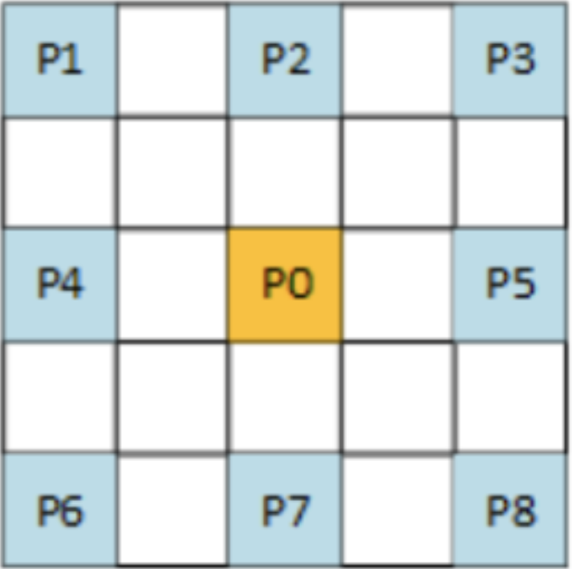
We can use this 3x3 average filter being applied to the pixel p7 and this 5x5 section of an image as an example.

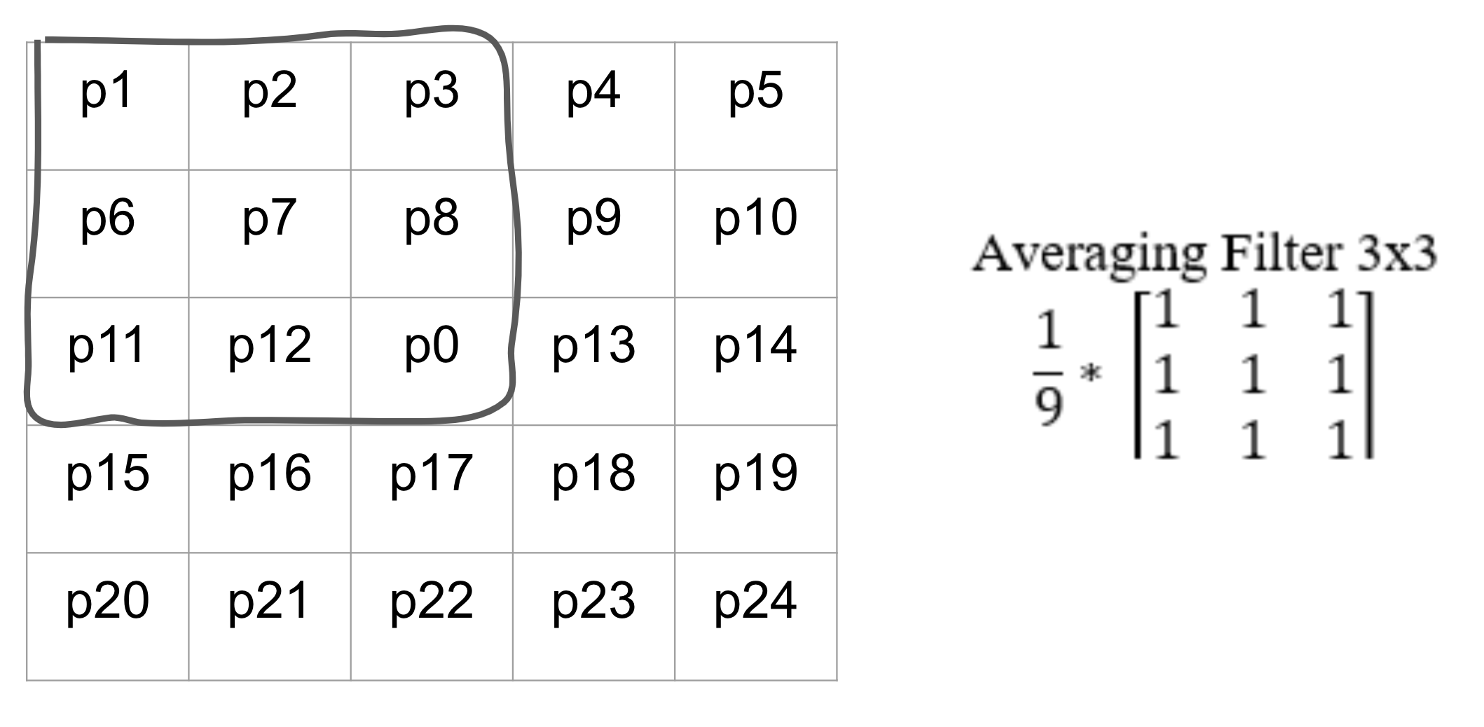
When applying filters, you always make a copy of the image first. After that, when the filter is being applied to the pixel p7, the outlined section would be extracted to create a 3x3 matrix. Then, the extracted portion of the image would be multiplied elementwise to the averaging filter. Finally, you would take the sum of all values in the resulting 3x3 matrix, and map that value back on to p7 in the copy of the image, not the original image.

Once p7 has been updated in the copied image, the filter moves on to the next pixel, p8.

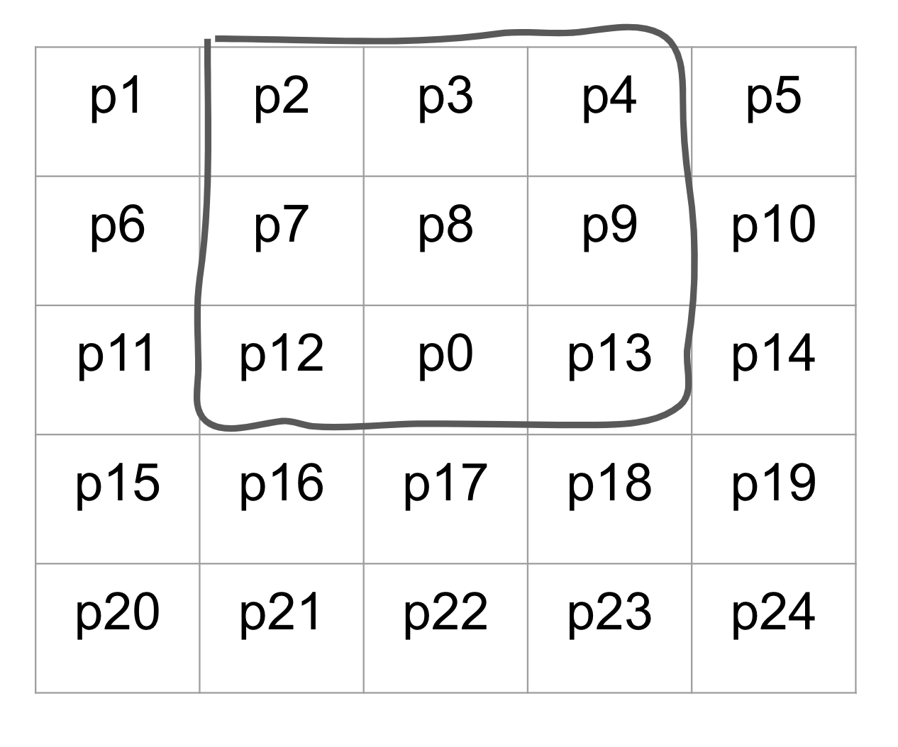
The process of applying the filter is the same as before, but the 3x3 area that is to be extracted from the image has changed. Most notably, p7 is now one of the values that is used in the calculation of the new p8 value. And this is the reason why we always update copies of the image, and we never update the original image directly. If we had changed the value of p7, the value of p7 being passed into p8's filter would be wrong. Then p9, p10, and all of the following pixels would have their input values being misrepresented.

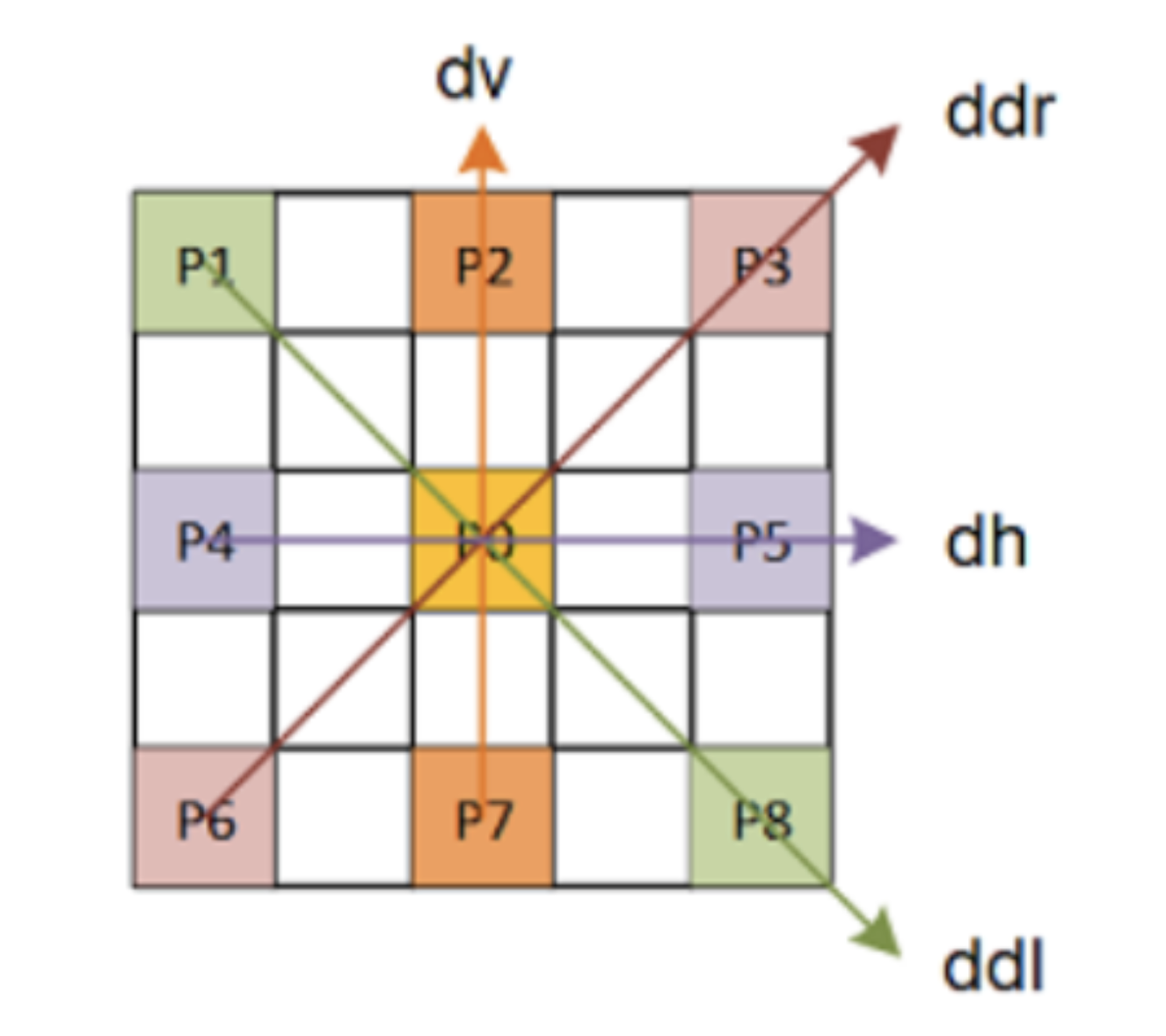
When we actually apply filters in our ISP, instead of looping through the image with nested for loops one pixel at a time, we will instead create a unique array for each value used in the filter. For example, for a 3x3 filter applied on a bayer image, we would extract the following arrays:

Now, the values at every index of the 9 arrays make up the values that would have been extracted by a 3x3 filter at the corresponding pixel. After that, we can stack up all of the arrays into a 3D array, and then take the sum across the new axis as shown below to finalize the filter.

There are various different types of filters, and they each serve their own purposes. The anti-aliasing filter is a preventative filter that is applied to images to prevent future noise from interpolations like color filter array interpolation

The types of noise that anti-aliasing filter prevents is referred to by the umbrella term aliasing noise. The most notable aliasing noise is blocky or jagged edges, and other types include false color artifacts and moire patterns.

Anti-Aliasing filters are generally in the following form, with a value of 1 for all of the neighboring pixels and a value of k with k>1 for the center pixel p0. k is a variable value that helps to determine the strength of the anti-aliasing.

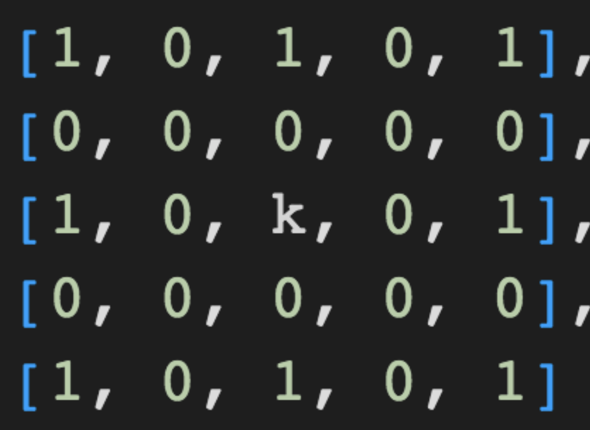
The 0's in the filter exist to ensure that filter only interacts with the same color neighbors of p0. This filter will smoothen out an image by applying an effect similar to an average filter, but by increasing or decreasing the value of k, you can set how much weight to give the center pixel.

We will use this image of a capital letter 'W' with blocky edges as an example to see the effects of anti-aliasing.

After applying the anti-aliasing filter with a k value of 12, we get this blurry W with smoother edges.

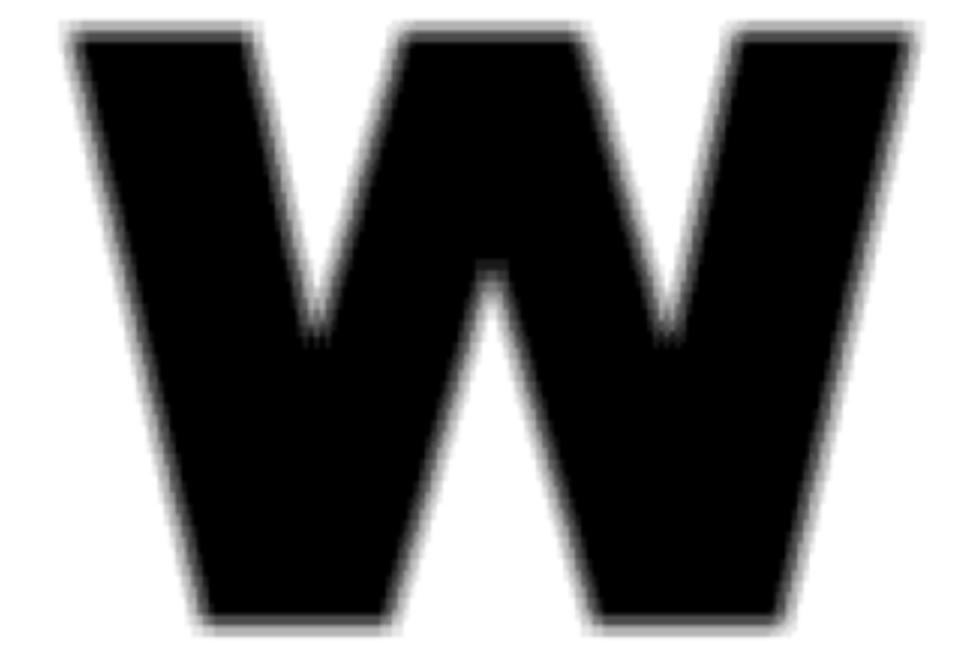
Since the resulting image is very blurry, we can see that the chosen k value was too extreme. In fact, k values are generally fairly small - a good general value to use is k=8. Despite that, we can easily see that the originally blocky edges have been smoothened out.

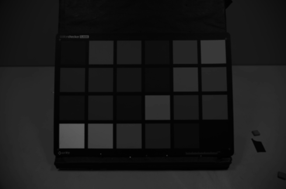
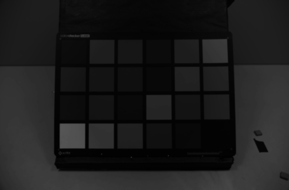
Lastly, we can apply the Anti-Aliasing Filter to the bayer image.

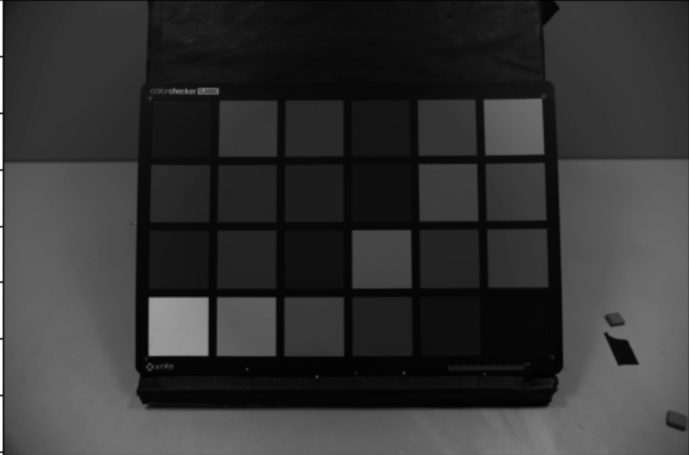
Resulting image after applying Anti-Aliasing Filter

Link to the AWB video

Link to the ___ video

Link to the ___ video

Link to the ___ video

Link to the ___ video

Link to the ___ video

Link to the ___ video

Link to the ___ video

Link to the ___ video